Fast thickmap ImageJ/Fiji plugin
This is documentation for the Fast thickmap ImageJ/Fiji plugin.
What does it do?
The Fast thickmap plugin calculates local thickness map of a binary image. Local thickness at \(\vec{x}\) is the diameter of the largest sphere that contains \(\vec{x}\) and fits into the foreground pixels. If the set of foreground pixels is denoted by \(\Omega\), the local thickness \(\tau\) is defined by
where \(S(\vec{p}, r)\) is a sphere centered at \(\vec{p}\) having radius \(r\).
The local thickness map can be used, e.g. to determine the diameter distribution of structures in the image.
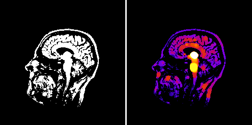
One slice of a binary input image (left) and its local thickness map (right). Brighter colors correspond to thicker regions.
Installation
Plain ImageJ
Download the latest .jar file from GitHub into Plugins folder of your ImageJ installation. Re-start ImageJ or use Help>Refresh menus command. The Fast thickmap plugin(s) are now installed into the Plugins>Fast thickmap submenu.
Fiji
Enable update site Fast thickmap (https://sites.imagej.net/AMiettinen/) and perform update. The Fast thickmap plugins will be installed into the Plugins>Fast thickmap submenu.
Usage
Make a binary image and then run Plugins>Fast Thickmap on it. The plugin will calculate the local thickness map of non-zero pixels.
In the settings dialog you can specify if you would like to use the integer radius approximation. The approximation makes processing even faster but the resulting thickness map will contain only integer values.
If the temporary data required by the plugin does not fit into the RAM of your computer, your image will be automatically processed in smaller chunks.
How it works?
The algorithm is described in [a]. Essentially, it follows the same procedure than the Hildebrand-Ruegsegger algorithm [b], but replaces its sphere plotting phase with a faster algorithm.
First, a distance map of the foreground pixels (non-zero pixels) is calculated. The distance map is then processed into a distance ridge. The distance ridge is a superset of the centers of maximal spheres that must be drawn in order to generate the thickness map. Each distance ridge point defines a sphere, and all the spheres are drawn using a separable algorithm. This results in a local squared radius map that is finally processed into the local thickness map.
The set of fast thickmap plugins includes all the above steps as separate plugins, and a driver plugin that does all of the steps at once.
The result is very similar to what can be done with the standard Hildebrand-Ruegsegger local thickness plugin [b], but
- the calculation is faster and
- the definition of a digital sphere is slightly different between the Hildebrand-Ruegsegger and the Fast thickmap plugins. Do not expect 100 % match in the results.
- As a downside, this faster algorithm requires more memory, but that is overcome by processing large images in smaller chunks as discussed above.
See also
A more performant implementation is available as a standalone program or Python package in the Pi2 software. An example and the documentation can be found here.
The original Hildebrand-Ruegsegger plugin can be found here or here.
License
If you use this plugin in scientific work, please cite [a].
This plugin is licensed under the GNU General Public License Version 3.
Bibliography
| [a] | (1, 2)
|
| [b] | (1, 2)
|